Note #4: An Introduction to t-SNE
17 Sep 2018Paper review: L.J.P. Maaten & G. Hinton, Visualizing Data using t-SNE, JMLR 2008
The intuition behind t-SNE
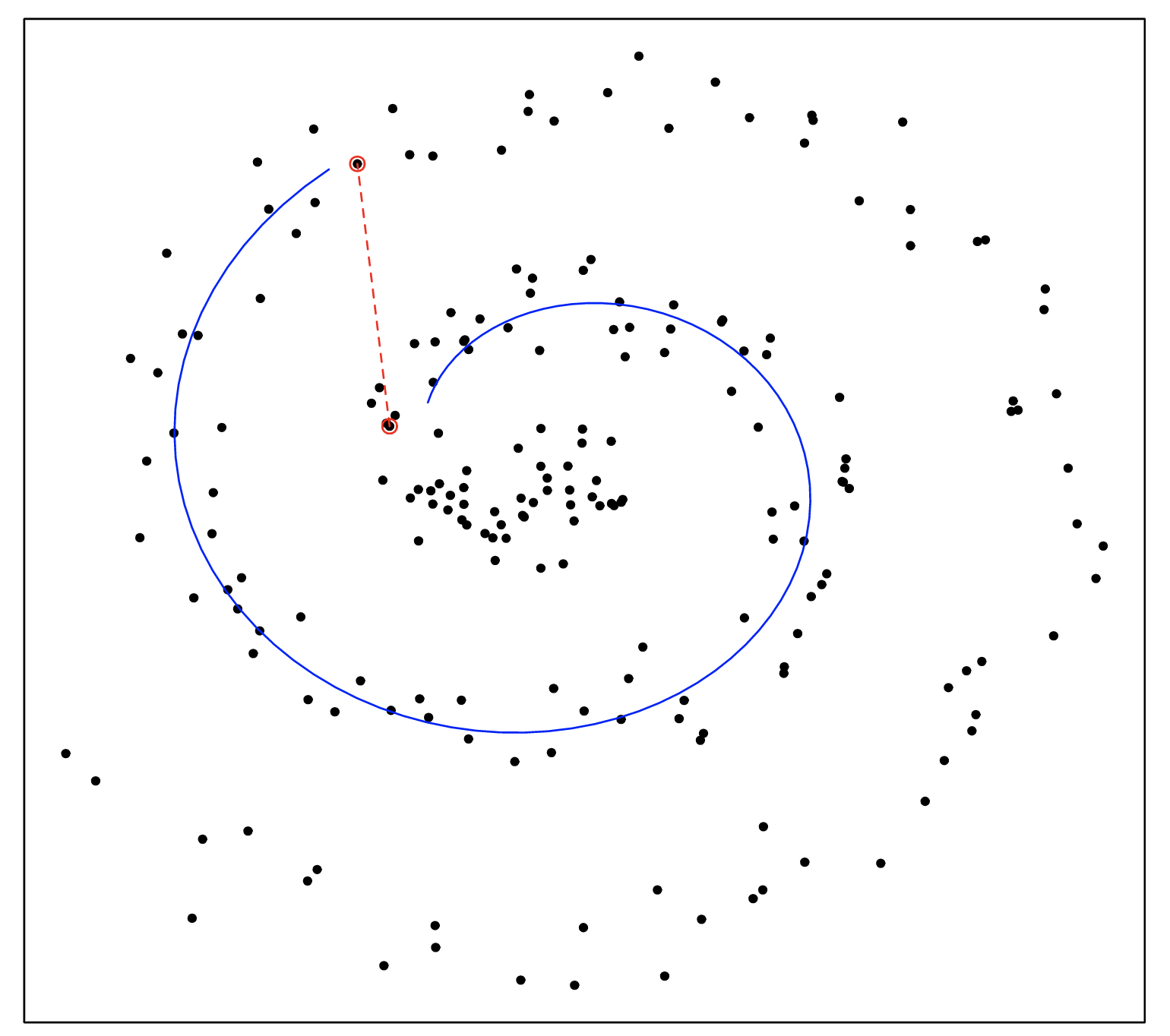
Traditional techniques such as PCA focus on finding a low-dimensional mapping of the data that maximally preserves variance. Hence, the squared distance measure favours correctly modeling large pairwise distances. However, large Euclidean distances between two points in high dimensions may not reliably reflect dissimilarities. In the Swiss roll below, the Euclidean distance between the two highlighted points does not accurately reflect how far apart they are on the manifold.

On the other hand, very small Euclidean distances accurately reflect points which are similar on the manifold. This is the focus of tSNE, which preserves local structure by:
- Modeling similar datapoints with small pairwise distances in the map
- Modeling dissimilar datapoints with large (and often amplified) pairwise distances
Cost function
The two objectives above are modeled into the cost function of t-SNE. First off, let’s define:

t-SNE aims to find a low-dimensional data representation that minimizes the mismatch between two probability distributions P and Q. This is done by minimizing their Kullback-Leibler (KL) divergence, resulting in the following cost function:

The behaviour of t-SNE can easily understood by examining four properties of the cost function.
Property 1: Non-convexity
Optimising the t-SNE cost function is trickier than traditional techniques like PCA because the cost function is non-convex. In practice, the cost function is minimised using gradient descent since the gradient can be computed analytically. However, different initialisations can result in quite different embeddings and optimisation is susceptible to local minima.
Property 2: Maps similar points close together
The cost function penalises two cases where a mismatch between P and Q occurs. Because the KL divergence is asymmetric, the penalty weight differs in the two cases:

Hence, we observe that t-SNE is focused on modeling similar points in high-dimensional space (high pij) with points that are close to each other in the low-dimensional map (high qij).
Property 3: Amplifies distances between dissimilar points
Nevertheless, dissimilar points should also be mapped far apart. In fact, t-SNE amplifies these distances because of the distribution chosen to model similarity between datapoints. P consists of the pairwise joint distribution pij which models the similarity between two points in the high-dimensional space. This gives the joint probability that the two points would pick each other as neighbours if a Gaussian probability distribution were centered around each point.
Likewise, Q models the similarity between two points in the low-dimensional map. However, instead of using a Gaussian, a Student-t distribution is centered around each point. Because the Student-t distribution is heavy-tailed compared to a Gaussian, for a low pij to be mapped to an equally low qij, dissimilar points must be pushed further apart in the low-dimensional map.
For this reason, t-SNE visualisations often provide clearer distinctions between dissimilar clusters. It also alleviates the crowding problem that occurs when a dataset of high intrinsic dimensionality (e.g. 10) is squeezed into an embedding space of lower dimensionality (e.g. 2).
Property 4: Computationally expensive
At every gradient descent step, the cost function evaluates the pairwise distances between all points. Hence, t-SNE has a computational and memory complexity that is quadratic in the number of datapoints. This makes standard t-SNE infeasible on datasets larger than ~10,000 points. The complexity cost is somewhat alleviated by a variant of t-SNE that uses the Barnes-Hut approximation.