Update #11

16 Jan 2019

Stochastic Training of Graph Convolution Nets (GCNs)

In the previous post, we saw that graph nets are capable of minimising the augmented tSNE loss on graph data. Here, we will explore an advantage of using a graph net instead of pure tSNE: we can make use of SGD to train our nets in mini-batches of data.

One reason why deep learning scales so well is the fact that networks can be trained using stochastic gradient descent (SGD). Recent work has shown that GCNs can be trained using SGD, albeit requiring additional tricks like importance sampling [Chen & Ma, 2018], or control variates [Chen, 2018].

In the following, we aim to train the network in mini-batches on the CORA citation network. In particular, the train set of 2,166 samples is randomly split into 12 mini-batches during each training epoch. The following augmentations were used to make SGD work.

Using 2 conv layers instead of 10

The receptive field of a node in a GCN with L layers is given by its L-hop neighborhood. It is unlikely that very distant neighbors are significant in a small graph like the CORA network, especially when taking mini-batches. Hence, I opted to use two graph convolutional layers, following the architecture in [Kipf & Welling, 2017].

Neighborhood averaging

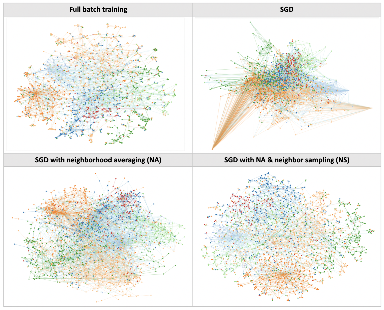
Using the original nets, we observe that the resulting projections are heavily distorted, especially in the case of nodes having high degrees. The problem is probably due to the fact that a given node sees much more of its neighbors when projecting on the complete graph (at test time) versus in a mini-batch (at training time).

This prompted me to change the neighborhood transfer function, such that the convolution takes a weighted average of neighbors’ activations, instead of a pure sum. The transfer function is now given by:

Neighbor sampling

Among the SGD training procedures for GCNs, neighbor sampling (NS) is the simplest to implement and originally used in GraphSAGE [Hamilton & Ying, 2017]. To reduce the receptive field size, NS randomly chooses D(l) neighbors for each node at layer l. The maximum receptive field size of each node is thus given by the product over all D(l). In the following experiment, we set D = [5, 10].