Update #5.5

28 Oct 2018

Pre-trained ResNet on CIFAR 10

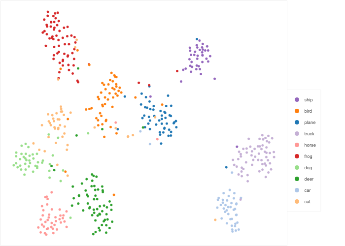
Here, we consider a pre-trained ResNet with 90% accuracy on CIFAR 10. Note that CIFAR 10 images have dimensionality 3 x 32 x 32. By taking the convolutional feature vectors of the penultimate layer, we obtain the feature matrix Z, given by a n x 64 matrix. Using t-SNE, we can visualize Z in two dimensions.

Finetuning on MNIST

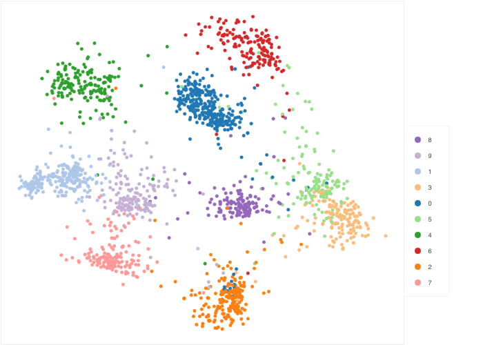
Next, we apply the same ResNet on MNIST images to obtain the feature matrix Z. Note that MNIST images have dimensionality 1 x 28 x 28. Visualising Z using t-SNE, we can see a fair amount of structure.

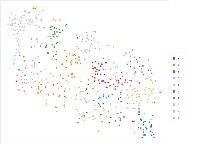
After finetuning the network, we achieve 95% classification accuracy on MNIST. The finetuned network yields feature vectors at the penultimate layer that provides much clearer structure. Visualising Z using t-SNE:

Learning t-SNE on Z for MNIST

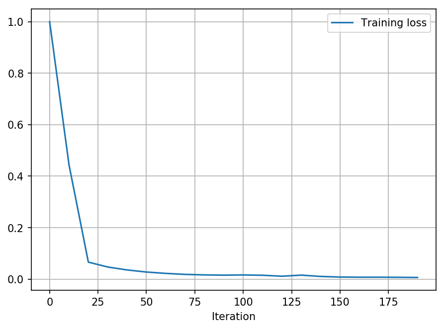
We use a graph net to learn a mapping from the feature matrix Z (n x 64) to the embedding matrix Y (n x 2). The graph net is trained using a set of 5,000 MNIST embeddings.

Transfer learning evaluation on USPS

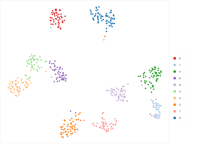
Lastly, we apply the pre-trained ResNet and the graph net on a test set of 1,860 USPS images. Note that USPS images have dimensionality 1 x 16 x 16. Using the same ResNet, we extract the feature matrix Z (n x 64). Using the same graph net, we obtain the embedding matrix Y (n x 2).

Here’s a visualisation of Y which shows a clear separation of classes!